---
bibliography: references.bib
---

# Mapping With R

## Types of maps

The fonction `mf_map()` is the central function of the package `mapsf` [@mapsf]. It makes it possible to carry out most of the usual representations in cartography. These main arguments are:

-   `x`, an sf object ;
-   `var`, the name of variable to present ;
-   `type`, the type of presentation.

### Create a simple map

The following lines import the spatial information layers located in the [geopackage](https://www.geopackage.org/) **cambodia.gpkg** file.

```{r, class.output="code-out", warning=FALSE, message=FALSE}
library(sf)

#Import Cambodia country border
country = st_read("data_cambodia/cambodia.gpkg", layer = "country", quiet = TRUE)
#Import provincial administrative border of Cambodia
education = st_read("data_cambodia/cambodia.gpkg", layer = "education", quiet = TRUE)
#Import district administrative border of Cambodia
district = st_read("data_cambodia/cambodia.gpkg", layer = "district", quiet = TRUE)
#Import roads data in Cambodia
road = st_read("data_cambodia/cambodia.gpkg", layer = "road", quiet = TRUE)
#Import health center data in Cambodia
hospital = st_read("data_cambodia/cambodia.gpkg", layer = "hospital", quiet = TRUE)

```

```{r mf_base, class.output="code-out", warning=FALSE, message=FALSE}
library(mapsf)

mf_map(x = district, border = "white")
mf_map(x = country,lwd = 2, col = NA, add = TRUE)
mf_map(x = road, lwd = .5, col = "ivory4", add = TRUE)
mf_map(x = hospital, pch = 20, cex = 1, col = "#FE9A2E", add = TRUE) 
```

### Proportional symbol map

Proportional symbol maps are used to represent inventory variables (absolute quantitative variables, sum and average make sense). The function `mf_map(..., type = "prop")` proposes this representation.

```{r proportional_symbols, class.output="code-out", warning=FALSE, message=FALSE}

#District
mf_map(x = district)     

# Proportional symbol 
mf_map(
  x = district, 
  var = "T_POP",
  val_max = 700000,
  type = "prop",
  col = "#148F77", 
  leg_title = "Population 2019"
)

# Title
mf_title("Distribution of population in provincial level")

```

#### Compare multiple map

It is possible to fix the dimensions of the largest symbol corresponding to a certain value with the arguments `inches` and `val_max`. We can use construct maps with comparable proportional symbols.

```{r proportional_symbols_comp, fig.height = 4, class.output="code-out", warning=FALSE, message=FALSE}
par(mfrow = c(1,2))   #Displaying two maps facing each other

#district
mf_map(x = district, border = "grey90", lwd = .5)    
# Add male Population
mf_map(
  x = district, 
  var = "Male", 
  type = "prop",
  col = "#1F618D",
  inches = 0.2, 
  val_max = 300000, 
  leg_title = "Male", 
  leg_val_cex = 0.5,
)
mf_title("Male Population by Distict")   #Adding map title

#district
mf_map(x = district, border = "grey90", lwd = .5)    
# Add female Population
mf_map(
  x = district, 
  var = "Female", 
  type = "prop",
  col = "#E74C3C",
  inches = 0.2, 
  val_max = 300000, 
  leg_title ="Female", 
  leg_val_cex = 0.5
)
mf_title("Female Population by Distict")     #Adding map title

```

Here we have displayed two maps facing each other, see the point [Displaying several maps on the same figure](#afficher-plusieurs-cartes-sur-la-même-figure) for more details.

### Choropleth map

Choropleth maps are used to represent ratio variables (relative quantitative variables, mean has meaning, sum has no meaning).

For this type of representation, you must first:

-   choose a discretization method to transform a continuous statistical series into classes defined by intervals,
-   choose a number of classes,
-   choose a color palette.

The function mf_map(..., type = "choro")makes it possible to create choroplete maps. The arguments nbreaks and breaks are used to parameterize the discretizations, and the function `mf_get_breaks()` makes it possible to work on the discretizations outside the function `mf_map()`. Similarly, the argument palis used to fill in a color palette, but several functions can be used to set the palettes apart from the (`mf_get_pal`...) function.

```{r choro, class.output="code-out", warning=FALSE, message=FALSE}
# Population density (inhabitants/km2) using the sf::st_area() function
district$DENS <- 1e6 * district$T_POP / as.numeric(st_area(district))   #Calculate population density 
mf_map(
  x = district,
  var = "DENS",
  type = "choro",
  breaks = "quantile",
  pal = "BuGn",
  lwd = 1,
  leg_title = "Distribution of population\n(inhabitants per km2)", 
  leg_val_rnd = 0
)
mf_title("Distribution of the population in (2019)")
```

```{r choro-incidence, class.output="code-out", warning=FALSE, message=FALSE, eval=TRUE}
cases = st_read("data_cambodia/cambodia.gpkg", layer = "cases", quiet = TRUE)
cases = subset(cases, Disease == "W fever")
population <- read.csv("data_cambodia/khm_admpop_adm2_2016_v2.csv")
population <- population[, c("ADM2_PCODE", "T_TL")]
# Remove commas
population$T_TL <- as.numeric(gsub(",","",population$T_TL))
district$cases <- lengths(st_intersects(district, cases))
district <- merge(district,
                  population,
                  by = "ADM2_PCODE")
district$incidence <- district$cases / district$T_TL * 100000

mf_map(x = district,
       var = "incidence",
       type = "choro",
       leg_title = "Incidence (per 100 000)")
mf_layout(title = "Incidence of W Fever in Cambodia")
```

#### Discretisation {#discretisation}

The fonction `mf_get_breaks()` provides the methods of discretization of classic variables: quantiles, average/standard deviation, equal amplitudes, nested averages, Fisher-Jenks, geometric, etc.

```{r discr2, fig.height=6, fig.width=8, class.output="code-out", warning=FALSE, message=FALSE}

education$enrol_g_pct = 100 * education$enrol_girl/education$t_enrol   #Calculate percentage of enrolled girl student

d1 = mf_get_breaks(education$enrol_g_pct, nbreaks = 6, breaks = "equal", freq = TRUE)
d2 = mf_get_breaks(education$enrol_g_pct, nbreaks = 6, breaks = "quantile")
d3 = mf_get_breaks(education$enrol_g_pct, nbreaks = 6, breaks = "geom")
d4 = mf_get_breaks(education$enrol_g_pct, breaks = "msd", central = FALSE)

```

```{r discr3, fig.height=6, fig.width=8, echo = FALSE, class.output="code-out", warning=FALSE, message=FALSE}

opar <- par(mfrow = c(2,2))
hist(education$enrol_g_pct, breaks = d1, main = "d1 : equal amplitudes")
rug(education$enrol_g_pct)

hist(education$enrol_g_pct, breaks = d2, main = "d2 : equal numbers")
abline(v = quantile(education$enrol_g_pct, probs = seq(0,1,length.out = 7)), col  = "red")
legend("topright", legend = "quantiles", col = "red", lty = 1, bty = "n")
rug(education$enrol_g_pct)

hist(education$enrol_g_pct, breaks = d3, main = "d3 :geometric progression")
rug(education$enrol_g_pct)

hist(education$enrol_g_pct, breaks = d4, main = "d4 : mean and standard deviation")
abline(v = mean(education$enrol_g_pct), col  = "red")
abline(v = mean(education$enrol_g_pct) + sd(education$enrol_g_pct), col  = "blue")
abline(v = mean(education$enrol_g_pct) - sd(education$enrol_g_pct), col  = "blue")
legend("topright", legend = c("mean", "mean +/-\n standard deviation"), col = c("red", "blue"), lty = 1, bty = "n")
rug(education$enrol_g_pct)
par(opar)

```

#### Color palettes {#palettes}

The argument `pal` de `mf_map()` is dedicated to choosing a color palette. The palettes provided by the function `hcl.colors()` can be used directly.

```{r pal1, fig.width = 6, fig.height = 6, class.output="code-out", warning=FALSE, message=FALSE}
mf_map(x = education, var = "enrol_g_pct", type = "choro",
       breaks = d3, pal = "Reds 3")
```

![](img/swatch-plot-1.svg){fig-align="center" width="600"}

The fonction `mf_get_pal()` allows you to build a color palette. This function is especially useful for creating balanced asymmetrical diverging palettes.

```{r pal2,  fig.height=3, nm=TRUE, class.output="code-out", warning=FALSE, message=FALSE}

mypal <- mf_get_pal(n = c(4,6), palette = c("Burg", "Teal"))
image(1:10, 1, as.matrix(1:10), col=mypal, xlab = "", ylab = "", xaxt = "n",
      yaxt = "n",bty = "n")

```

#### For a point layer

It is possible to use this mode of presentation in specific implementation also.

```{r choropt, class.output="code-out", warning=FALSE, message=FALSE}
dist_c <- st_centroid(district)
mf_map(district)
mf_map(
  x = dist_c,
  var = "DENS",
  type = "choro",
  breaks = "quantile",
  nbreaks = 5,
  pal = "PuRd",
  pch = 23,
  cex = 1.5,
  border = "white",
  lwd = .7,
  leg_pos = "topleft",
  leg_title = "Distribution of population\n(inhabitants per km2)", 
  leg_val_rnd = 0, 
  add = TRUE
)
mf_title("Distribution of population in (2019)")

```

### Typology map

Typology maps are used to represent qualitative variables. The function `mf_map(..., type = "typo")` proposes this representation.

```{r typo_simple, class.output="code-out", warning=FALSE, message=FALSE}
mf_map(
  x = district,
  var="Status",
  type = "typo",
  pal = c('#E8F9FD','#FF7396','#E4BAD4','#FFE3FE'),
  lwd = .7,
  leg_title = ""
)
mf_title("Administrative status by size of area")
```

#### Ordering value in the legend

The argument `val_order` is used to order the categories in the

```{r typo_order, class.output="code-out", warning=FALSE, message=FALSE}
mf_map(
  x = district,
  var="Status",
  type = "typo",
  pal = c('#E8F9FD','#FF7396','#E4BAD4','#FFE3FE'),
  val_order = c("1st largest district", "2nd largest district", "3rd largest district","<4500km2"),
  lwd = .7,
  leg_title = ""
)
mf_title("Administrative status by size of area")
```

#### Map of point

When the implantation of the layer is punctual, symbols are used to carry the colors of the typology.

```{r typo_point, class.output="code-out", warning=FALSE, message=FALSE}
#extract centroid point of the district
dist_ctr <- st_centroid(district[district$Status != "<4500km2", ])
mf_map(district)
mf_map(
  x = dist_ctr,
  var = "Status",
  type = "typo",
  cex = 2,
  pch = 22,
  pal = c('#FF7396','#E4BAD4','#FFE3FE'),
  leg_title = "",
  leg_pos = "bottomright",
  add = TRUE
)
mf_title("Administrative status by size of area")

```

#### Map of lines

```{r, class.output="code-out", warning=FALSE, message=FALSE}
#Selection of roads that intersect the city of Siem Reap
pp <- district[district$ADM1_EN == "Phnom Penh", ]
road_pp <- road[st_intersects(x = road, y = pp, sparse = FALSE), ]
mf_map(pp)
mf_map(
  x = road_pp,
  var = "fclass",
  type = "typo",
  lwd = 1.2,
  pal = mf_get_pal(n = 6, "Tropic"),
  leg_title = "Types of road",
  leg_pos = "topright",
  leg_frame = T,
  add = TRUE
)
mf_title("Administrative status")
```

### Map of stocks and ratios

The function `mf_map(..., var = c("var1", "var2"), type = "prop_choro")` represents proportional symbols whose areas are proportional to the values of one variable and whose color is based on the discretization of a second variable. The function uses the arguments of the functions `mf_map(..., type = "prop")` and `mf_map(..., type = "choro")`.

```{r choroprop, class.output="code-out", warning=FALSE, message=FALSE}
mf_map(x = district)
mf_map(
  x = district,
  var = c("T_POP", "DENS"),
  val_max = 500000,
  type = "prop_choro",
  border = "grey60",
  lwd = 0.5,
  leg_pos = c("bottomright", "bottomleft"),
  leg_title = c("Population", "Density of\n population\n(inhabitants per km2)"),
  breaks = "q6",
  pal = "Blues 3",
  leg_val_rnd = c(0,1))
mf_title("Population")
```

### Map of stocks and categories

The function `mf_map(..., var = c("var1", "var2"), type = "prop_typo")` represents proportional symbols whose areas are proportional to the values of one variable and whose color is based on the discretization of a second variable. The function uses the arguments of the `mf_map(..., type = "prop")` and function `mf_map(..., type = "typo")`.

```{r typoprop, class.output="code-out", warning=FALSE, message=FALSE}
mf_map(x = district)
mf_map(
  x = district,
  var = c("Area.Km2.", "Status"),
  type = "prop_typo",
  pal = c('#E8F9FD','#FF7396','#E4BAD4','#FFE3FE'),
  val_order = c("<4500km2","1st largest district", "2nd largest district", "3rd largest district"),
  leg_pos = c("bottomleft","topleft"),
  leg_title = c("Population\n(2019)",
                "Statut administratif"),
)
mf_title("Population")
```

## Layout

To be finalized, a thematic map must contain certain additional elements such as: title, author, source, scale, orientation...

### Example data

The following lines import the spatial information layers located in the [geopackage](https://www.geopackage.org/) **cambodia.gpkg** file.

```{r, class.output="code-out", warning=FALSE, message=FALSE}
library(sf)
country = st_read("data_cambodia/cambodia.gpkg", layer = "country", quiet = TRUE)         #Import Cambodia country border
education = st_read("data_cambodia/cambodia.gpkg", layer = "education", quiet = TRUE)     #Import provincial administrative border of Cambodia
district = st_read("data_cambodia/cambodia.gpkg", layer = "district", quiet = TRUE)       #Import district administrative border of Cambodia
road = st_read("data_cambodia/cambodia.gpkg", layer = "road", quiet = TRUE)               #Import roads data in Cambodia
hospital = st_read("data_cambodia/cambodia.gpkg", layer = "hospital", quiet = TRUE)       #Import hospital data in Cambodia
cases = st_read("data_cambodia/cambodia.gpkg", layer = "cases", quiet = TRUE)             #Import example data of fever_cases in Cambodia

```

### Themes

The function `mf_theme()` defines a cartographic theme. Using a theme allows you to define several graphic parameters which are then applied to the maps created with `mapsf`. These parameters are: the map margins, the main color, the background color, the position and the aspect of the title. A theme can also be defined with the `mf_init()` and function `mf_export()`.

#### Use a predefined theme

A series of predefined themes are available by default (see `?mf_theme`).

```{r them1, fig.show='hold', fig.width =8, fig.height = 8, class.output="code-out", warning=FALSE, message=FALSE}
library(mapsf)
# use of a background color for the figure, to see the use of margin
opar <- par(mfrow = c(2,2))
# Using a predefined theme
mf_theme("default")
mf_map(district)
mf_title("Theme : 'default'")

mf_theme("darkula")
mf_map(district)
mf_title("Theme : 'darkula'")

mf_theme("candy")
mf_map(district)
mf_title("Theme : 'candy'")

mf_theme("nevermind")
mf_map(district)
mf_title("Theme : 'nevermind'")
par(opar)

```

#### Modify an existing theme

It is possible to modify an existing theme. In this example, we are using the "default" theme and modifying a few settings.

```{r theme2, fig.width = 8, fig.height = 4, fig.show='hold', class.output="code-out", warning=FALSE, message=FALSE}
library(mapsf)
opar <- par(mfrow = c(1,2))
mf_theme("default")
mf_map(district)
mf_title("default")

mf_theme("default", tab = FALSE, font = 4, bg = "grey60", pos = "center")
mf_map(district)
mf_title("modified default")
par(opar)
```

#### Create a theme

It is also possible to create a theme.

```{r, class.output="code-out", warning=FALSE, message=FALSE}
mf_theme(
  bg = "lightblue",    # background color
  fg = "tomato1",      # main color
  mar = c(1,0,1.5,0),  # margin
  tab = FALSE,         # "tab" style for the title
  inner = FALSE,       # title inside or outside of map area
  line = 1.5,          # space dedicated to title
  pos = "center",      # heading position
  cex = 1.5,           # title size
  font = 2             # font types for title
)
mf_map(district)
mf_title("New theme")
```

### Titles

The function `mf_title()` adds a title to a map.

```{r, class.output="code-out", warning=FALSE, message=FALSE}
mf_theme("default")
mf_map(district)
mf_title("Map title")
```

It is possible to customize the appearance of the title

```{r, class.output="code-out", warning=FALSE, message=FALSE}
mf_map(district)
mf_title(
  txt = "Map title", 
  pos = "center", 
  tab = FALSE, 
  bg = "tomato3", 
  fg = "lightblue", 
  cex = 1.5, 
  line = 1.7, 
  font = 1, 
  inner = FALSE
)
```

### Arrow orientation

The function `mf_arrow()` allows you to choose the position and aspect of orientation arrow.

```{r north, class.output="code-out", warning=FALSE, message=FALSE}
mf_map(district)
mf_arrow()
```

### Scale

The function `mf_scale()` allows you to choose the position and the aspect of the scale.

```{r scale, class.output="code-out", warning=FALSE, message=FALSE}

mf_map(district)
mf_scale(
  size = 60,
  lwd = 1,
  cex = 0.7
)

```

### Credits

The function `mf_credits()` displays a line of credits (sources, author, etc.).

```{r credit, class.output="code-out", warning=FALSE, message=FALSE}
mf_map(district)
mf_credits("IRD\nInstitut Pasteur du Cambodge, 2022")
```

### Complete dressing

The function `mf_layout()` displays all these elements.

```{r layout1, class.output="code-out", warning=FALSE, message=FALSE}
mf_map(district)
mf_layout(
  title = "Cambodia",
  credits = "IRD\nInstitut Pasteur du Cambodge, 2022",
  arrow = TRUE
)
```

### Annotations

```{r, class.output="code-out", warning=FALSE, message=FALSE}
mf_map(district)
mf_annotation(district[district$ADM2_EN == "Bakan",], txt = "Bakan", col_txt = "darkred", halo = TRUE, cex = 1.5)

```

### Legends

```{r, class.output="code-out", warning=FALSE, message=FALSE}
mf_map(district)
mf_legend(
  type = "prop", 
  val = c(1000,500,200,10), 
  inches = .2, 
  title = "Population", 
  pos = "topleft"
)
mf_legend(
  type = "choro", 
  val = c(0,10,20,30,40),
  pal = "Greens", 
  pos = "bottomright", 
  val_rnd = 0
)

```

### Labels

The function `mf_label()` is dedicated to displaying labels.

```{r labs, class.output="code-out", warning=FALSE, message=FALSE}
dist_selected <- district[st_intersects(district, district[district$ADM2_EN == "Bakan", ], sparse = F), ]

mf_map(dist_selected)
mf_label(
  x = dist_selected,
  var = "ADM2_EN",
  col= "darkgreen",
  halo = TRUE,
  overlap = FALSE, 
  lines = FALSE
)
mf_scale()
```

The argument `halo = TRUE` allows to display a slight halo around the labels and the argument `overlap = FALSE` allows to create non-overlapping labels.

### Center the map on a region

The function `mf_init()` allows you to initialize a map by centering it on a spatial object.

```{r, class.output="code-out", warning=FALSE, message=FALSE}
mf_init(x = dist_selected)
mf_map(district, add = TRUE)
mf_map(dist_selected, col = NA, border = "#29a3a3", lwd = 2, add = TRUE)
```

### Displaying several maps on the same figure

Here you have to use `mfrow` of the function `par()`. The first digit represents the number of of rows and second the number of columns.

```{r mfrow0, fig.width=7, fig.height = 3.5,  eval = TRUE, class.output="code-out", warning=FALSE, message=FALSE}
# define the figure layout (1 row, 2 columns)
par(mfrow = c(1, 2))

# first map
mf_map(district)
mf_map(district, "Male", "prop", val_max = 300000)
mf_title("Population, male")

# second map
mf_map(district)
mf_map(district, "Female", "prop", val_max = 300000)
mf_title("Population, female")
```

### Exporting maps

It is quite difficult to export figures (maps or others) whose height/width ratio is satisfactory. The default ratio of figures in png format is 1 (480x480 pixels):

```{r, results='hide', class.output="code-out", warning=FALSE, message=FALSE}
dist_filter <- district[district$ADM2_PCODE == "KH0808", ]
png("img/dist_filter_1.png")
mf_map(dist_filter)
mf_title("Filtered district")
dev.off()
```

![](img/dist_filter_1.png){fig-align="center"}

On this map a lot of space is lost to the left and right of the district.

The function `mf_export()` allows exports of maps whose height/width ratio is controlled and corresponds to that of a spatial object.

```{r, results='hide', class.output="code-out", warning=FALSE, message=FALSE}
mf_export(dist_filter, "img/dist_filter_2.png", width = 480)
mf_map(dist_filter)
mf_title("Filtered district")
dev.off()
```

![](img/dist_filter_2.png){fig-align="center" width="218"}

The extent of this map is exactly that of the displayed region.

### Adding an image to a map

This can be useful for adding a logo, a pictograph. The function `readPNG()` of package `png` allows the additional images on the figure.

```{r logo, class.output="code-out", warning=FALSE, message=FALSE}
mf_theme("default", mar = c(0,0,0,0))
library(png)

logo <- readPNG("img/ird_logo.png")       #Import image
pp <- dim(logo)[2:1]*200                           #Image dimension in map unit (width and height of the original image)

#The upper left corner of the department's bounding box
xy <- st_bbox(district)[c(1,4)]
mf_map(district, col = "#D1914D", border = "white")
rasterImage(
  image   = logo,
  xleft   = xy[1] ,
  ybottom = xy[2] - pp[2],
  xright  = xy[1] + pp[1],
  ytop    = xy[2]
)

```

### Place an item precisely on the map

The function `locator()` allows clicking on the figure and obtaining the coordinate of a point in the coordinate system of the figure (of the map).

```{Place texts or items on map}
# locator(1)                                      # click to get coordinate on map
# points(locator(1))                              # click to plot point on map
# text(locator(1),                                # click to place the item on map
#      labels ="Located any texts on map",        
#      adj = c(0,0))

```

![](img/locator.webm)

`locator()`peut être utilisée sur la plupart des graphiques (pas ceux produits avec `ggplot2`).

::: {.callout-note appearance="minimal" icon="false"}
[How to interactively position legends and layout elements on a map with cartography](https://rgeomatic.hypotheses.org/1837)
:::

### Add shading to a layer

The function `mf_shadow()` allows to create a shadow to a layer of polygons.

```{r shadow, class.output="code-out", warning=FALSE, message=FALSE}
mf_shadow(district)
mf_map(district, add=TRUE)

```

### Creating Boxes

The function `mf_inset_on()` allows to start creation a box. You must then "close" the box with `mf_inset_off()`.

```{r inset, fig.width = 6.5, fig.height = 5, class.output="code-out", warning=FALSE, message=FALSE}

mf_init(x = dist_selected, theme = "agolalight", expandBB = c(0,.1,0,.5)) 
mf_map(district, add = TRUE)
mf_map(dist_selected, col = "tomato4", border = "tomato1", lwd = 2, add = TRUE)

# Cambodia inset box
mf_inset_on(x = country, pos = "topright", cex = .3)
mf_map(country, lwd = .5, border= "grey90")
mf_map(dist_selected, col = "tomato4", border = "tomato1", lwd = .5, add = TRUE)
mf_scale(size = 100, pos = "bottomleft", cex = .6, lwd = .5)
mf_inset_off()

# District inset box
mf_inset_on(x = district, pos = "bottomright", cex = .3)
mf_map(district, lwd = 0.5, border= "grey90")
mf_map(dist_selected, col = "tomato4", border = "tomato1", lwd = .5, add = TRUE)
mf_scale(size = 100, pos = "bottomright", cex = .6, lwd = .5)
mf_inset_off()

# World inset box
mf_inset_on(x = "worldmap", pos = "topleft")
mf_worldmap(dist_selected, land_col = "#cccccc", border_col = NA, 
            water_col =  "#e3e3e3", col = "tomato4")

mf_inset_off()
mf_title("Bakan district and its surroundings")
mf_scale(10, pos = 'bottomleft')

```

## 3D maps

### linemap

The package `linemap` [@linemap] allows you to make maps made up of lines.

```{r linemap, class.output="code-out", warning=FALSE, message=FALSE}
library(linemap)
library(mapsf)
library(sf)
library(dplyr)

pp = st_read("data_cambodia/PP.gpkg", quiet = TRUE)      # import Phnom Penh administrative border
pp_pop_dens <- getgrid(x = pp, cellsize =1000, var = "DENs")   # create population density in grid format  (pop density/1km)

mf_init(pp)

linemap(
  x = pp_pop_dens,  
  var = "DENs",
  k = 1,
  threshold = 5, 
  lwd = 1,
  col = "ivory1",
  border = "ivory4",
  add = T)

mf_title("Phnom Penh Population Density, 2019")
mf_credits("Humanitarian Data Exchange, 2022\nunit data:km2")


# url = "https://data.humdata.org/dataset/1803994d-6218-4b98-ac3a-30c7f85c6dbc/resource/f30b0f4b-1c40-45f3-986d-2820375ea8dd/download/health_facility.zip"
# health_facility.zip = "health_facility.zip"
# download.file(url, destfile = health_facility.zip)
# unzip(health_facility.zip) # Unzipped files are in a new folder named Health
# list.files(path="Health")

```

### Relief Tanaka

We use the `tanaka` package [@tanaka] which provides a method [@tanaka1950] used to improve the perception of relief.

```{r tanaka, class.output="code-out", warning=FALSE, message=FALSE}
library(tanaka)
library(terra)

rpop <- rast("data_cambodia/khm_pd_2019_1km_utm.tif")     # Import population raster data (in UTM)
district = st_read("data_cambodia/cambodia.gpkg", layer = "district", quiet = TRUE)   # Import Cambodian districts layer
district <- st_transform(district, st_crs(rpop))    # Transform data into the same coordinate system

mat <- focalMat(x = rpop, d = c(1500), type = "Gauss")  # Raster smoothing
rpopl <- focal(x = rpop, w = mat, fun = sum, na.rm = TRUE)

# Mapping
cols <- hcl.colors(8, "Reds", alpha = 1, rev = T)[-1]
mf_theme("agolalight")
mf_init(district)
tanaka(x = rpop, breaks = c(0,10,25,50,100,250,500,64265),
       col = cols, add = T, mask = district, legend.pos = "n")
mf_legend(type = "choro", pos = "bottomright", 
          val = c(0,10,25,50,100,250,500,64265), pal = cols,
          bg = "#EDF4F5", fg = NA, frame = T, val_rnd = 0,
          title = "Population\nper km2")
mf_title("Population density of Cambodia, 2019")
mf_credits("Humanitarian Data Exchange, 2022",
           bg = "#EDF4F5")

```

::: {.callout-note appearance="minimal" icon="false"}
[The tanaka package](https://rgeomatic.hypotheses.org/1758)
:::

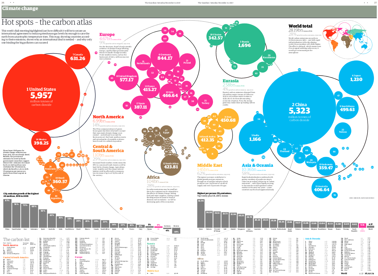
## Cartographic Transformation

> classical anamorphosis is a representation of States(or any cells) by **rectangle or any polygons** according to a **quantities** attached to them. (...) We strive to **keep the general arrangement** of meshes or the silhouette of the continent."\
> @Brunet93

3 types of anamorphoses or cartograms are presented here:

-   Dorling's cartograms [@Dorling96]
-   Non-contiguous cartograms [@Olson76]
-   Contiguous cartograms [@Dougenik85]

::: {.callout-note appearance="minimal" icon="false"}
A comprehensive course on anamorphoses : [Les anamorphoses cartographiques](https://neocarto.hypotheses.org/366) [@Lambert15].
:::

::: {.callout-note appearance="minimal" icon="false"}
[Make cartograms with R](https://rgeomatic.hypotheses.org/1361)
:::

To make the cartograms we use the package `cartogram` [@cartogram].

### Dorling's cartograms

The territories are represented by figures (circles, squares or rectangles) which do not overlap, the surface of which are proportional to a variable. The proportion of the figures are defined according to the starting positions.

![](img/dorling.png){fig-align="center" width="600"}

```{block2, type='rmdmoins'}
Space is quite poorly identified.  
You can name the circles to get your bearings and/or use the color to make clusters appear and better identify the geographical blocks.
```

```{block2, type='rmdplus'}
The perception of quantities is very good. The circle sizes are really comarable.
```

```{r dorling, class.output="code-out", warning=FALSE, message=FALSE}
library(mapsf)
library(cartogram)
district <- st_read("data_cambodia/cambodia.gpkg", layer = "district" , quiet = TRUE)
dist_dorling <- cartogram_dorling(x = district, weight = "T_POP", k = 0.7)
mf_map(dist_dorling, col = "#40E0D0", border= "white")
mf_label(
  x = dist_dorling[order(dist_dorling$T_POP, decreasing = TRUE), ][1:10,], 
  var = "ADM2_EN",
  overlap = FALSE, 
  # show.lines = FALSE,
  halo = TRUE, 
  r = 0.15
)
mf_title("Population of District - Dorling Cartogram")
```

The parameter `k` allows to vary the expansion factor of the circles.

### Non-continuous cartograms

The size of the polygons is proportional to a variable. The arrangement of the polygons relative to each other is preserved. The shape of the polygons is similar.

![](img/nccartogram.png){fig-align="center"}

[@Cauvin13]

```{block2, type='rmdmoins'}
The topology of the regions is lost.
```

```{block2, type='rmdplus'}
The converstion of the polygons shape is optimal.
```

```{r olson, class.output="code-out", warning=FALSE, message=FALSE}
dist_ncont <- cartogram_ncont(x = district, weight = "T_POP", k = 1.2)
mf_map(district, col = NA, border = "#FDFEFE", lwd = 1.5)
mf_map(dist_ncont, col = "#20B2AA", border= "white", add = TRUE)
mf_title("Population of District - Non-continuous cartograms")
```

The parameter `k` allows to vary the expansion of the polygons.

### Continuous cartograms

The size of the polygons is proportional to variable. The arrangement of the polygons relative to each other is preserved. To maintain contiguity, the sape of the polygons is heavily transformed.

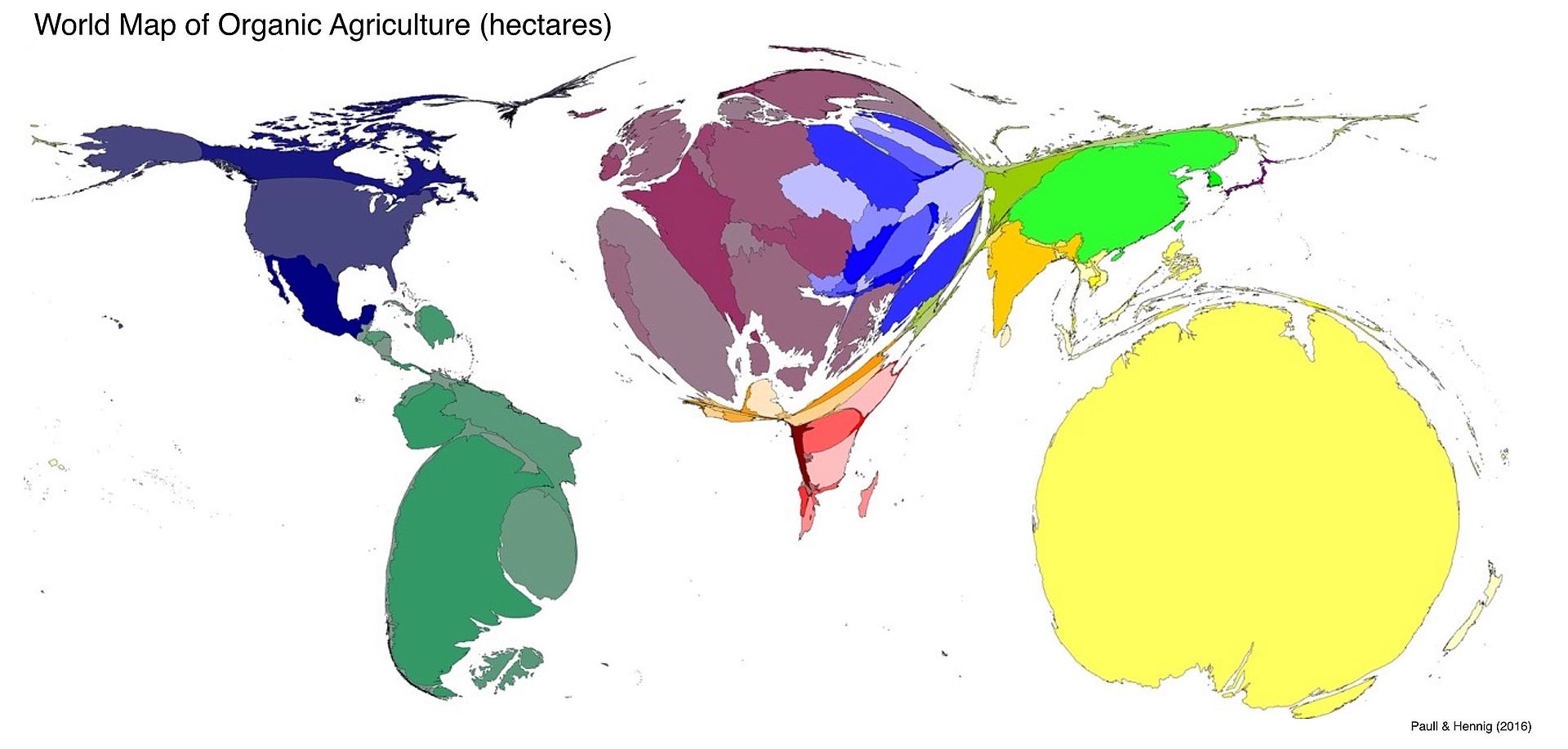![](img/cartogram.jpg){fig-align="center" width="600"}

[@Paull16]

```{block2, type='rmdmoins'}
The shape of the polygond is strongly distorted.
```

```{block2, type='rmdplus'}

It is a "real geographical map": topology and contiguity are preserved.

```

```{r dougenik}
dist_ncont <- cartogram_cont(x = district, weight = "DENs", maxSizeError = 6)
mf_map(dist_ncont, col = "#66CDAA", border= "white", add = FALSE)
mf_title("Population of District - Continuous cartograms")
mf_inset_on(district, cex = .2, pos = "bottomleft")
mf_map(district, lwd = .5)
mf_inset_off()
```

### Stengths and weaknessses of cartograms

cartograms are cartographic representations perceived as **innovative** (although the method is 40 years old). These very generalize images capture **quantities** and **gradients** well. These are real **communication** images that **provoke**, arouse **interest**, convey a strong **message**, **challenge**.

But cartograms induce a loss of **visual cues** (difficult to find one's country or region on the map), require a **reading effort** which can be significant and do not make it possible to manage **missing data**.