# Work with Raster Data
This chapter is largely inspired by two presentation; @MmadelinSIGR and @JNowosadSIGR; carried out as part of the [SIGR2021](https://sigr2021.github.io/site/index.html) thematic school.
## Format of objects `SpatRaster`
The package `terra` [@terra] allows to handle vector and raster data. To manipulate this spatial data, `terra` store it in object of type `SpatVector` and `SpatRaster`. In this chapter, we focus on the manipulation of raster data (`SpatRaster`) from functions offered by this package.
An object `SpatRaster` allows to handle vector and raster data, in one or more layers (variables). This object also stores a number of fundamental parameters that describe it (number of columns, rows, spatial extent, coordinate reference system, etc.).
![Source : [@RasterCheatSheet]](img/raster.png){fig-align="center" width="350"}
## Importing and exporting data
The package `terra` allows importing and exporting raster files. It is based on the [GDAL](https://gdal.org/) library which makes it possible to read and process a very large number of geographic image formats.
```{r terra, message=FALSE}
library(terra)
```
The function `rast()` allows you to create and/or import raster data. The following lines import the raster file **elevation.tif** ([*Tagged Image File Format*](https://fr.wikipedia.org/wiki/Tagged_Image_File_Format)) into an object of type `SpatRaster` (default).
```{r import_raster, message=FALSE}
elevation <- rast("data_cambodia/elevation.tif")
elevation
```
Modifying the name of the stored variable (altitude).
```{r names_raster, message=FALSE}
names(elevation) <- "Altitude"
```
The function `writeRaster()` allow you to save an object `SpatRaster` on your machine, in the format of your choice.
```{r export_raster, eval=FALSE}
writeRaster(x = elevation, filename = "data_cambodia/new_elevation.tif")
```
## Displaying a SpatRaster object
The function `plot()` is use to display an object `SpatRaster`.
```{r affichage_1_raster, eval=TRUE, fig.align='center', fig.width=6}
plot(elevation)
```
A raster always contains numerical data, but it can be both quantitative data and numerically coded qualitative (categorical) data (ex: type of land cover).
Specify the type of data stored with the augment `type` (`type = "continuous"` default), to display them correctly.
Import and display of raster containing categorical data: Phnom Penh Land Cover 2019 (land cover types) with a resolution of 1.5 meters:
```{r import_raster_2, message=FALSE}
lulc_2019 <- rast("data_cambodia/lulc_2019.tif") #Import Phnom Penh landcover 2019, landcover types
```
The landcover data was produced from SPOT7 satellite image with 1.5 meter spatial resolution. An extraction centered on the municipality of Phnom Penh was then carried out.
```{r affichage_raster_2, fig.align='center', fig.width=6}
plot(lulc_2019, type = "classes")
```
To display the actual tiles of landcover types, as well as the official colors of Phnom Penh Landcover nomenclature (available [here](https://www.statistiques.developpement-durable.gouv.fr/corine-land-cover-0)), you can proceed as follows.
```{r affichage_raster_3, eval=TRUE, fig.align='center', fig.width = 12}
class_name <- c(
"Roads",
"Built-up areas",
"Water Bodies and rivers",
"Wetlands",
"Dry bare area",
"Bare crop fields",
"Low vegetation areas",
"High vegetation areas",
"Forested areas")
class_color <- c("#070401", "#c84639", "#1398eb","#8bc2c2",
"#dc7b34", "#a6bd5f","#e8e8e8", "#4fb040", "#35741f")
plot(lulc_2019,
type = "classes",
levels = class_name,
col = class_color,
plg = list(cex = 0.7),
mar = c(3.1, 3.1, 2.1, 10) #The margin are (bottom, left, top, right) respectively
)
```
## Change to the study area
### (Re)projections {#reprojections}
To modify the projection system of a raster, use the function `project()`. It is then necessary to indicate the method for estimating the new cell values.
{fig-align="center"}
Four interpolation methods are available:
- ***near*** : nearest neighbor, fast and default method for qualitative data;\
- ***bilinear*** : bilinear interpolation. Default method for quantitative data;\
- ***cubic*** : cubic interpolation;\
- ***cubicspline*** : cubic spline interpolation.
```{r reproj_raster, eval=TRUE, fig.align='center', fig.width=8}
# Re-project data
elevation_utm = project(x = elevation, y = "EPSG:32648", method = "bilinear") #from WGS84(EPSG:4326) to UTM zone48N(EPSG:32648)
lulc_2019_utm = project(x = lulc_2019, y = "EPSG:32648", method = "near") #keep original projection: UTM zone48N(EPSG:32648)
```
```{r reproj_raster_2, eval=TRUE, echo=FALSE, fig.align='center', fig.width = 7}
par(mfrow=c(1,2))
plot(elevation_utm, main="Projected elevation raster in UTM 48 N" )
plot(lulc_2019_utm, type ="classes", main="CLC 2018 projected in UTM 48 N")
```
### Crop {#crop}
Clipping a raster to the extent of another object `SpatVector` or `SpatRaster` is achievable with the `crop()`.
::: {layout-ncol="2"}
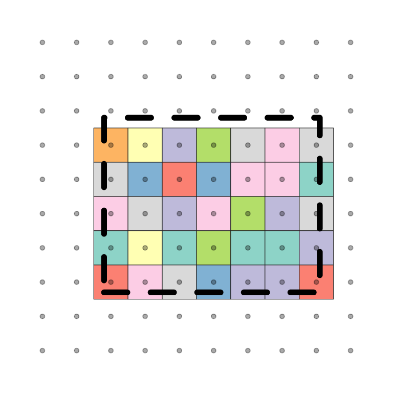
Source : [@RasterCheatSheet]
:::
Import vector data of (municipal divisions) using function `vect`. This data will be stored in an `SpatVector` object.
```{r crop_raster, eval=TRUE}
district <- vect("data_cambodia/cambodia.gpkg", layer="district")
```
Extraction of district boundaries of Thma Bang district (ADM2_PCODE : KH0907).
```{r crop_raster_1, eval=TRUE}
thma_bang <- subset(district, district$ADM2_PCODE == "KH0907")
```
Using the function `crop()`, Both data layers must be in the same projection.
```{r crop_raster_3, eval=TRUE, fig.align='center', fig.width=6}
crop_thma_bang <- crop(elevation_utm, thma_bang)
plot(crop_thma_bang)
plot(thma_bang, add=TRUE)
```
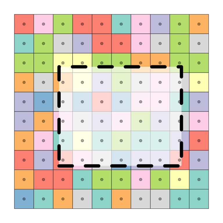
### Mask {#mask}
To display only the values of a raster contained in a polygon, use the function `mask()`.
![Source : [@RasterCheatSheet]](img/mask.png){fig-align="center" width="350"}
Creation of a mask on the **crop_thma_bang** raster to the municipal limits (polygon) of **Thma Bang district**.
```{r mask_raster, eval=TRUE, fig.align='center', fig.width=6}
mask_thma_bang <- mask(crop_thma_bang, thma_bang)
plot(mask_thma_bang)
plot(thma_bang, add = TRUE)
```
### Aggregation and disaggregation
Resampling a raster to a different resolution is done in two steps.
::: {layout-ncol="3"}

Source : [@RasterCheatSheet]
:::
Display the resolution of a raster with the function `res()`.
```{r agr_raster, eval=TRUE}
res(elevation_utm) #check cell size
```
Create a grid with the same extent, then decrease the spatial resolution (larger cells).
```{r agr_raster_1, eval=TRUE}
elevation_LowerGrid <- elevation_utm
# elevation_HigherGrid <- elevation_utm
res(elevation_LowerGrid) <- 1000 #cells size = 1000 meter
# res(elevation_HigherGrid) <- 10 #cells size = 10 meter
elevation_LowerGrid
```
The function `resample()` allows to resample the atarting values in the new spatial resolution. Several resampling methods are available (cf. [partie 5.4.1](#reprojections)).
```{r agr_raster_2, eval=TRUE, fig.align='center', fig.width=6}
elevation_LowerGrid <- resample(elevation_utm,
elevation_LowerGrid,
method = "bilinear")
plot(elevation_LowerGrid,
main="Cell size = 1000m\nBilinear resampling method")
```
### Raster fusion
Merge multiple objects `SpatRaster` into one with `merge()` or `mosaic()`.
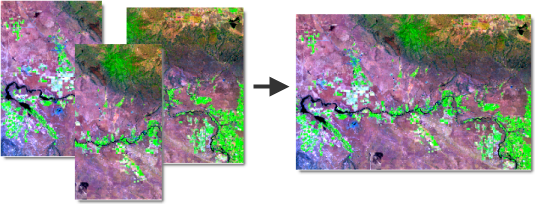{fig-align="center"}
After cutting the elevation raster by the municipal boundary of Thma Bang district (cf [partie 5.4.2](#crop)), we do the same thing for the neighboring municipality of Phnum Kravanh district.
```{r merge_raster, eval=TRUE}
phnum_kravanh <- subset(district, district$ADM2_PCODE == "KH1504") # Extraction of the municipal boundaries of Phnum Kravanh district
crop_phnum_kravanh <- crop(elevation_utm, phnum_kravanh) #clipping the elevation raster according to district boundaries
```
The **crop_thma_bang** and **crop_phnum_kravanh** elevation raster overlap spatially:
```{r merge_raster_1, eval=TRUE, echo=FALSE, fig.align='center',fig.width=8}
par(mfrow=c(1,2), mar=c(0,0,0,0))
plot(crop_thma_bang, main="Crop Thma Bang")
plot(thma_bang, add=TRUE)
plot(phnum_kravanh, add=TRUE)
plot(crop_phnum_kravanh, main="Crop Phnum Kravanh")
plot(phnum_kravanh, add=TRUE)
plot(thma_bang, add=TRUE)
```
The difference between the functions `merge()` and `mosiac()` relates to values of the overlapping cells. The function `mosaic()` calculate the average value while `merge()` holding the value of the object `SpaRaster` called n the function.
```{r merge_raster_2, eval=TRUE, fig.align='center', fig.width=6}
#in this example, merge() and mosaic() give the same result
merge_raster <- merge(crop_thma_bang, crop_phnum_kravanh)
mosaic_raster <- mosaic(crop_thma_bang, crop_phnum_kravanh)
plot(merge_raster)
# plot(mosaic_raster)
```
### Segregate
Decompose a raster by value (or modality) into different rasterlayers with the function `segregate`.
```{r segregate, eval=TRUE, fig.align='center', fig.width=6}
lulc_2019_class <- segregate(lulc_2019, keep=TRUE, other=NA) #creating a raster layer by modality
plot(lulc_2019_class)
```
## Map Algebra
Map algebra is classified into four groups of operation [@Tomlin_1990]:
- ***Local*** : operation by cell, on one or more layers;\
- ***Focal*** : neighborhood operation (surrounding cells);\
- ***Zonal*** : to summarize the matrix values for certain zones, usually irregular;
- ***Global*** : to summarize the matrix values of one or more matrices.
![Source : [@XingongLi2009]](img/lo_fo_zo_glo.png){fig-align="center"}
### Local operations
![Source : [@JMennis2015]](img/op_local_2.png){fig-align="center" width="452"}
#### Value replacement
```{r op_local_0, eval=FALSE}
elevation_utm[elevation_utm[[1]]== -9999] <- NA #replaces -9999 values with NA
elevation_utm[elevation_utm < 1500] <- NA #Replace values < 1500 with NA
```
```{r op_local_00, eval=TRUE}
elevation_utm[is.na(elevation_utm)] <- 0 #replace NA values with 0
```
#### Operation on each cell
```{r op_local_1, eval=TRUE}
elevation_1000 <- elevation_utm + 1000 # Adding 1000 to the value of each cell
elevation_median <- elevation_utm - global(elevation_utm, median)[[1]] # Removed median elevation to each cell's value
```
```{r op_local_2, eval=TRUE, echo=FALSE, fig.align='center', fig.width=8}
par(mfrow=c(1,2), mar=c(0,0,0,0))
plot(elevation_1000, main="elevation_1000\nelevation + 1000")
plot(elevation_median, main="elevation_median\nelevation - median value")
```
#### Reclassification
Reclassifying raster values can be used to discretize quantitative data as well as to categorize qualitative categories.
```{r reclass_2, eval=TRUE}
reclassif <- matrix(c(1, 2, 1,
2, 4, 2,
4, 6, 3,
6, 9, 4),
ncol = 3, byrow = TRUE)
```
Values between 1 and 2 will be replaced by the value 1.\
Values between 3 and 4 will be replaced by the value 2.\
Values between 5 and 6 will be replaced by the value 3. Values between 7 and 9 will be replaced by the value 4.
...
```{r reclass_3, eval=TRUE}
reclassif
```
The function `classify()` allows you to perform the reclassification.
```{r reclass_4, eval=TRUE}
lulc_2019_reclass <- classify(lulc_2019, rcl = reclassif)
plot(lulc_2019_reclass, type ="classes")
```
Display with the official titles and colors of the different categories.
```{r reclass_6, eval=TRUE, fig.align='center', out.width="80%"}
plot(lulc_2019_reclass,
type ="classes",
levels=c("Urban areas",
"Water body",
"Bare areas",
"Vegetation areas"),
col=c("#E6004D",
"#00BFFF",
"#D3D3D3",
"#32CD32"),
mar=c(3, 1.5, 1, 11))
```
#### Operation on several layers (ex: NDVI)
It is possible to calculate the value of a cell from its values stored in different layers of an object `SpatRaster`.
Perhaps the most common example is the calculation of the [Normalized Vegetation Index (*NDVI*)](http://www.trameverteetbleue.fr/outils-methodes/donnees-mobilisables/indice-vegetation-modis). For each cell, a value is calculated from two layers of raster from a multispectral satellite image.
```{r NDVI, eval=TRUE}
# Import d'une image satellite multispectrale
sentinel2a <- rast("data_cambodia/Sentinel2A.tif")
```
This multispectral satellite image (10m resolution) dated 25/02/2020, was produced by Sentinel-2 satellite and was retrieved from [plateforme Copernicus Open Access Hub](https://scihub.copernicus.eu/dhus/#/home). An extraction of Red and near infrared spectral bands, centered on the Phnom Penh city, was then carried out.
```{r NDVI_1, eval=TRUE, fig.align='center', fig.width=7}
plot(sentinel2a)
```
To lighten the code, we assign the two matrix layers in different `SpatRaster` objects.
```{r NDVI_2, eval=TRUE}
B04_Red <- sentinel2a[[1]] #spectral band Red
B08_NIR <-sentinel2a[[2]] #spectral band near infrared
```
From these two raster objects , we can calculate the normalized vegetation index:
$${NDVI}=\frac{\mathrm{NIR} - \mathrm{Red}} {\mathrm{NIR} + \mathrm{Red}}$$
```{r NDVI_3, eval=TRUE, fig.align='center', out.width="90%"}
raster_NDVI <- (B08_NIR - B04_Red ) / (B08_NIR + B04_Red )
plot(raster_NDVI)
```
The higher the values (close to 1), the denser the vegetation.
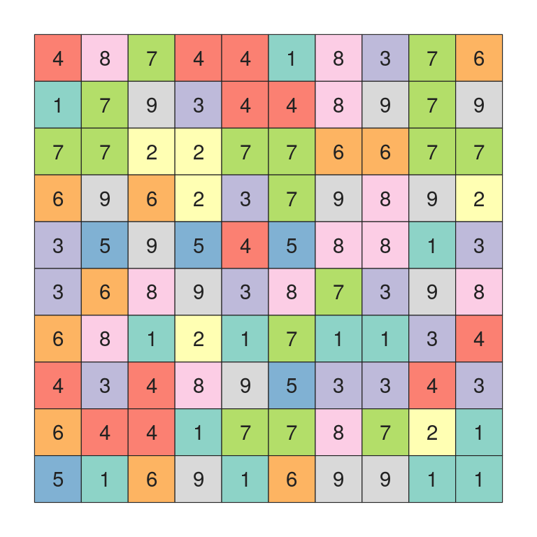
### Focal operations
![Source : [@JMennis2015]](img/op_focal_2.png){fig-align="center" width="415"}
Focal analysis conisders a cell plus its direct neighbors in contiguous and symmetrical (neighborhood operations). Most often, the value of the output cell is the result of a block of 3 x 3 (odd number) input cells.
The first step is to build a matrix that determines the block of cells that will be considered around each cell.
```{r op_focal_1, eval=TRUE}
# 5 x 5 matrix, where each cell has the same weight
mon_focal <- matrix(1, nrow = 5, ncol = 5)
mon_focal
```
The function `focal()` Then allows you to perform the desired analysis. For example: calculating the average of the values of all contiguous cells, for each cell in the raster.
```{r op_focal_3, eval=TRUE}
elevation_LowerGrid_mean <- focal(elevation_LowerGrid,
w = mon_focal,
fun = mean)
```
```{r op_focal_5, eval=TRUE, echo=FALSE, fig.align='center', fig.width=8}
par(mfrow=c(1,2), mar=c(0,0,0,0))
plot(elevation_LowerGrid, main="Elevation_LowerGrid\n(starting raster)")
plot(elevation_LowerGrid_mean, main="Elevation_LowerGrid_mean\n(focal result 5 x 5)")
```
#### Focal operations for elevation rasters
The function `terrain()` allows to perform focal analyzes specific to elevation rasters. Six operations are available:
- ***slope*** = calculation of the slope or degree of inclination of the surface;\
- ***aspect*** = calculate slope orientation;\
- ***roughness*** = calculate of the variability or irregularity of the elevation;\
- ***TPI*** = calculation of the index of topgraphic positions;\
- ***TRI*** = elevation variability index calculation;\
- ***flowdir*** = calculation of the water flow direction.
Example with calculation of slopes(*slope*).
```{r op_focal_6, eval=TRUE, fig.align='center', fig.width=6}
#slope calculation
slope <- terrain(elevation_utm, "slope",
neighbors = 8, #8 (or 4) cells around taken into account
unit = "degrees") #Output unit
plot(slope) #Inclination of the slopes, in degrees
```
### Global operations
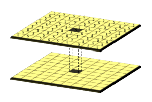{fig-align="center" width="297"}
Global operation are used to summarize the matrix values of one or more matrices.
```{r op_global_1, eval=TRUE}
global(elevation_utm, fun = "mean") #average values
```
```{r op_global_2, eval=TRUE}
global(elevation_utm, fun = "sd") #standard deviation
```
```{r op_global_3, eval=TRUE}
freq(lulc_2019_reclass) #frequency
table(lulc_2019_reclass[]) #contingency table
```
Statistical representations that summarize matrix information.
```{r op_global_4, eval=TRUE, fig.align='center', fig.width=6}
hist(elevation_utm) #histogram
density(elevation_utm) #density
```
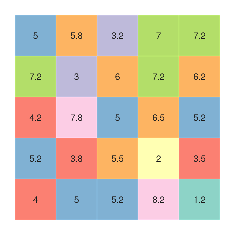
### Zonal operation
![Source : [@JMennis2015]](img/op_zonal_2.png){fig-align="center" width="342"}
The zonal operation make it possible to summarize the matrix values of certain zones (group of contiguous cells in space or in value).
#### Zonal operation on an extraction
**All global operations can be performed on an extraction of cells resulting from the functions `crop()`, `mask()`, `segregate()`...**
Example: average elevation for the city of Thma Bang district (cf [partie 5.4.3](#mask)).
```{r op_global_6, eval=TRUE}
# Average value of the "mask" raster over Thma Bang district
global(mask_thma_bang, fun = "mean", na.rm=TRUE)
```
#### Zonal operation from a vector layer
The function `extract()` allows you to extract and manipulate the values of cells that intersect vector data.
Example from polygons:
```{r op_zonal_poly, eval=TRUE}
# Average elevation for each polygon (district)?
elevation_by_dist <- extract(elevation_LowerGrid, district, fun=mean)
head(elevation_by_dist, 10)
```
#### Zonal operation from raster
Zonal operation can be performed by area bounded by the categorical values of a second raster. For this, the two raster must have exaclty the same extent and the same resolution.
```{r op_zonal_1, eval=TRUE}
#create a second raster with same resolution and extent as "elevation_clip"
elevation_clip <- rast("data_cambodia/elevation_clip.tif")
elevation_clip_utm <- project(x = elevation_clip, y = "EPSG:32648", method = "bilinear")
second_raster_CLC <- rast(elevation_clip_utm)
#resampling of lulc_2019_reclass
second_raster_CLC <- resample(lulc_2019_reclass, second_raster_CLC, method = "near")
#added a variable name for the second raster
names(second_raster_CLC) <- "lulc_2019_reclass_resample"
```
```{r op_zonal_2, eval=TRUE, echo=FALSE, fig.align='center', fig.width=8}
par(mfrow=c(1,2), mar=c(0,0,0,0))
plot(elevation_clip_utm, main="elevation_clip_utm")
plot(second_raster_CLC, type = "classes", main="lulc_2019_reclass_resample")
```
Calculation of the average elevation for the different areas of the second raster.
```{r op_zonal_3, eval=TRUE}
#average elevation for each area of the "second_raster"
zonal(elevation_clip_utm, second_raster_CLC , "mean", na.rm=TRUE)
```
## Transformation and conversion
### Rasterization
Convert polygons to raster format.
```{r Raster_vec1, eval=TRUE}
chamkarmon = subset(district, district$ADM2_PCODE =="KH1201")
raster_district <- rasterize(x = chamkarmon, y = elevation_clip_utm)
```
```{r Raster_vec11, eval=TRUE, fig.align='center', fig.width=6}
plot(raster_district)
```
Convert points to raster format
```{r Raster_vec2, eval=TRUE}
#rasterization of the centroids of the municipalities
raster_dist_centroid <- rasterize(x = centroids(district),
y = elevation_clip_utm, fun=sum)
plot(raster_dist_centroid, col = "red")
plot(district, add =TRUE)
```
Convert lines in raster format
```{r Raster_vec3, eval=TRUE}
#rasterization of municipal boundaries
raster_dist_line <- rasterize(x = as.lines(district), y = elevation_clip_utm, fun=sum)
```
```{r Raster_vec33, eval=TRUE}
plot(raster_dist_line)
```
### Vectorisation
Transform a raster to vector polygons.
```{r Raster_vec4, eval=TRUE}
polygon_elevation <- as.polygons(elevation_clip_utm)
```
```{r Raster_vec44, eval=TRUE}
plot(polygon_elevation, y = 1, border="white")
```
Transform a raster to vector points.
```{r Raster_vec5, eval=TRUE}
points_elevation <- as.points(elevation_clip_utm)
```
```{r Raster_vec55, eval=TRUE}
plot(points_elevation, y = 1, cex = 0.3)
```
Transform a raster into vector lines.
```{r Raster_vec6, eval=TRUE}
lines_elevation <- as.lines(elevation_clip_utm)
```
```{r Raster_vec66, eval=TRUE}
plot(lines_elevation)
```
### terra, raster, sf, stars...
Reference packages for manipulating spatial data all rely o their own object class. It is sometimes necessary to convert these objects from one class to another class to take advance of all the features offered by these different packages.
Conversion functions for raster data:
| FROM/TO | raster | terra | stars |
|---------|----------|--------------------------|---------------|
| raster | | rast() | st_as_stars() |
| terra | raster() | | st_as_stars() |
| stars | raster() | as(x, 'Raster') + rast() | |
Conversion functions for vector data:
| FROM/TO | sf | sp | terra |
|---------|------------|------------------|--------|
| sf | | as(x, 'Spatial') | vect() |
| sp | st_as_sf() | | vect() |
| terra | st_as_sf() | as(x, 'Spatial') | |